2  Visualizing the data

Note

Again, please note that data paths are relative to the root of the GitHub repository

Warning

This chapter requires data from Section 1.3 to be loaded!

## extra packages
require(ggimage)
require(packcircles)
require(ggrepel)
require(cowplot)
require(extrafont)

The most worn looks

## map hex colour to outfit
dressColorMapping <- unique(surpriseSongsDressColours %>% select(DressName, ColourHex1))
colorPaletteDresses <- setNames(dressColorMapping$ColourHex1, dressColorMapping$DressName)
pathToDressColours <- "dress_drawings/"
## map outfits to the corresponding images
oneRowPerConcert %>%
    count(DressName) %>%
    mutate(
        percentage = n / sum(n) * 100,
        imagePath = case_when(
            DressName == "Pink" ~paste0(pathToDressColours, "Pink.png"),
            DressName == "Green" ~paste0(pathToDressColours, "Green.png"),
            DressName == "Yellow" ~paste0(pathToDressColours, "Yellow.png"),
            DressName == "Blue" ~paste0(pathToDressColours, "Blue.png"),
            DressName == "Flamingo pink" ~ paste0(pathToDressColours,"Flamingo pink.png"),
            DressName == "Ocean blue" ~ paste0(pathToDressColours,"Ocean blue.png"),
            DressName == "Sunset orange" ~ paste0(pathToDressColours,"Sunset orange.png"),
            DressName == "Cotton candy" ~paste0(pathToDressColours, "Cotton candy.png"),
            DressName == "Blurple" ~paste0(pathToDressColours, "Blurple.png"),
            DressName == "Grapefruit" ~ paste0(pathToDressColours,"Grapefruit.png"),
            DressName == "Popsicle" ~ paste0(pathToDressColours,"Popsicle.png"),
            TRUE ~ NA_character_
        )) -> outfits

## barchart
ggplot(outfits, aes(x = reorder(DressName, -n), y = n, fill = DressName)) +
    geom_bar(stat = "identity", width = 0.8) +  
    geom_image(
        aes(image = imagePath, y = n),  
        size = 0.15,                    
        by = "height"                    
    ) +
    geom_text(
        aes(y = n + 3.8, label = paste0(n, "\n(", round(percentage, 1), "%)")),  
        vjust = 0,  
        color = "black",
        size = 4
    ) +
    scale_fill_manual(values = colorPaletteDresses) +
    theme_minimal() +
    labs(title = "", x = "", y = "") +
    theme(
        axis.text.x = element_text(angle = 45, hjust = 1, size = 14),
        axis.text.y = element_text(size = 14),
        plot.title = element_text(hjust = 0.5, size = 16),
        axis.title.x = element_blank(),
        axis.title.y = element_blank(),
        legend.position = "none"
    ) + ylim(0, 35)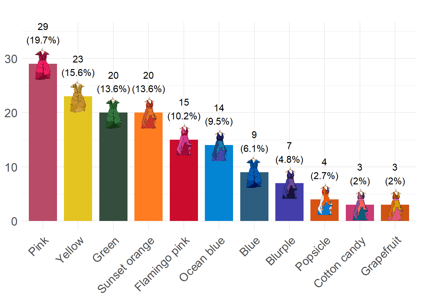

Eras’ Outfits and Special Events

dress_first_appearance <- surpriseSongsDressColours %>%
  group_by(DressName) %>%
  summarize(FirstAppearance = min(Date)) %>%
  arrange((FirstAppearance))
surpriseSongsDressColours$DressName <- factor(surpriseSongsDressColours$DressName,
                                              levels = dress_first_appearance$DressName)
max_dress_level <- length(unique(surpriseSongsDressColours$DressName))
dress_levels <- levels(factor(surpriseSongsDressColours$DressName))
outfits$DressName <- factor(outfits$DressName, levels = dress_levels)

main_plot <- ggplot(oneRowPerConcert, aes(x = Date, y = DressName, colour = ColourHex1)) +
  geom_point(size = 4, alpha = 1) +
  scale_colour_identity() +
  theme_minimal() +
  labs(x = "", y = "") +
  geom_rect(aes(xmin = as.Date("2023-08-28"), xmax = as.Date("2023-11-08"),
                ymin = -Inf, ymax = Inf), fill = "gray", alpha = 0.01, colour = NA) +
  geom_rect(aes(xmin = as.Date("2023-11-27"), xmax = as.Date("2024-02-06"),
                ymin = -Inf, ymax = Inf), fill = "gray", alpha = 0.01, colour = NA) +  
  geom_rect(aes(xmin = as.Date("2024-03-10"), xmax = as.Date("2024-05-08"),
                ymin = -Inf, ymax = Inf), fill = "gray", alpha = 0.01, colour = NA) +
  geom_rect(aes(xmin = as.Date("2024-08-21"), xmax = as.Date("2024-10-17"),
                ymin = -Inf, ymax = Inf), fill = "gray", alpha = 0.01, colour = NA) +
  # Vertical lines for the key events
  geom_vline(xintercept = as.Date("2024-05-09"), linetype = "dashed", colour = "black") +
  geom_vline(xintercept = as.Date("2023-03-17"), linetype = "dashed", colour = "black") +
  geom_vline(xintercept = as.Date("2024-10-18"), linetype = "dashed", colour = "black") +
  geom_vline(xintercept = as.Date("2023-08-24"), linetype = "dashed", colour = "black") +
  geom_vline(xintercept = as.Date("2024-02-07"), linetype = "dashed", colour = "black") +
  geom_vline(xintercept = as.Date("2024-04-16"), linetype = "solid", colour = "darkgray", size=2) +
  geom_vline(xintercept = as.Date("2023-07-07"), linetype = "solid", colour = "purple", size=2) +
  geom_vline(xintercept = as.Date("2023-10-27"), linetype = "solid", colour = "blue", size=2) +

  annotate("text", x = as.Date("2024-05-09"), y = max_dress_level, 
           label = "Europeᵃ", colour = "black", angle = -90, vjust = -0.5, family = "Calibri", size = 6, lineheight = 0.6) +
  annotate("text", x = as.Date("2023-03-17"), y = max_dress_level, 
           label = "United\n Statesᵃ", colour = "black", angle = -90, vjust = -0.2, family = "Calibri", size = 6, lineheight = 0.6) +
  annotate("text", x = as.Date("2024-10-18"), y = max_dress_level, 
           label = "North\n Americaᵃ", colour = "black", angle = -90, vjust = -0.2, family = "Calibri", size = 6, lineheight = 0.6) +
  annotate("text", x = as.Date("2023-08-24"), y = max_dress_level, 
           label = "Latin\n Americaᵃ", colour = "black", angle = -90, vjust = -0.2, family = "Calibri", size = 6, lineheight = 0.6) +
  annotate("text", x = as.Date("2024-02-07"), y = max_dress_level, 
           label = "Asia/\n Oceaniaᵃ", colour = "black", angle = -90, vjust = -0.2, family = "Calibri", size = 6, lineheight = 0.6) +
  annotate("text", x = as.Date("2024-04-16"), y = max_dress_level, 
           label = "TTPDᵇ", colour = "darkgray", angle = -90, vjust = -0.5, family = "Calibri", size = 6, lineheight = 0.6,
           fontface = "bold") +
  annotate("text", x = as.Date("2023-07-07"), y = max_dress_level, 
           label = "    Speak Now\nTVᵇ", colour = "purple", angle = -90, vjust = -0.2, family = "Calibri", size = 6, lineheight = 0.6) +
  annotate("text", x = as.Date("2023-10-27"), y = max_dress_level, 
           label = "1989\nTVᵇ", colour = "blue", angle = -90, vjust = -0.2, family = "Calibri", size = 6, lineheight = 0.6) +
  scale_x_date(date_labels = "%b %Y", date_breaks = "3 months") +
  theme(
    axis.text.x = element_text(angle = 0, hjust = 1, size = 16),
    axis.text.y = element_blank(),
    axis.ticks.y = element_blank(),
    plot.title = element_text(hjust=0.5, size = 14, margin = margin(b = 20), face = "bold"),
    plot.margin = margin(t = 0, r = 0, b = 10, l = 0),
    text = element_text(colour = "black", family = "Calibri", size = 16)
  )

count_plot <- ggplot(outfits, aes(x = n, y = DressName, fill = DressName)) +
  geom_bar(stat = "identity", width = 0.8) +
  geom_image(
    aes(image = imagePath, x = n),  
    size = 0.095,                    
    nudge_x = 0.5,
    by = "height"                    
  ) +
  geom_text(
    aes(x = n + 3, label = paste0(n, " (", round(percentage, 1), "%) - ", DressName)),  # Added dress name
    hjust = 0,
    nudge_x = 3.5,
    colour = "black",
    size = 6,
    family = "Calibri"
  ) +
  scale_fill_manual(values = colorPaletteDresses) +
  theme_minimal() +
  labs(title = "", x = "", y = "") +
  theme(
    axis.text = element_blank(),
    axis.ticks = element_blank(),  # Remove any remaining ticks
    plot.title = element_text(hjust = 0.5, size = 12),
    legend.position = "none",
    plot.margin = margin(t = 0, r = 0, b = 10, l = 0),
    text = element_text(colour = "black", family = "Calibri", size = 16)
  ) +
  xlim(0, 65)   # Increased limit to accommodate longer text with dress names

# Merge the plots using cowplot with adjusted widths
merged_plot <- plot_grid(
  count_plot, main_plot,
  ncol = 2,
  align = "h",
  axis = "tb",
  rel_widths = c(2, 3)  # Increased count plot width to accommodate longer text
)


merged_plot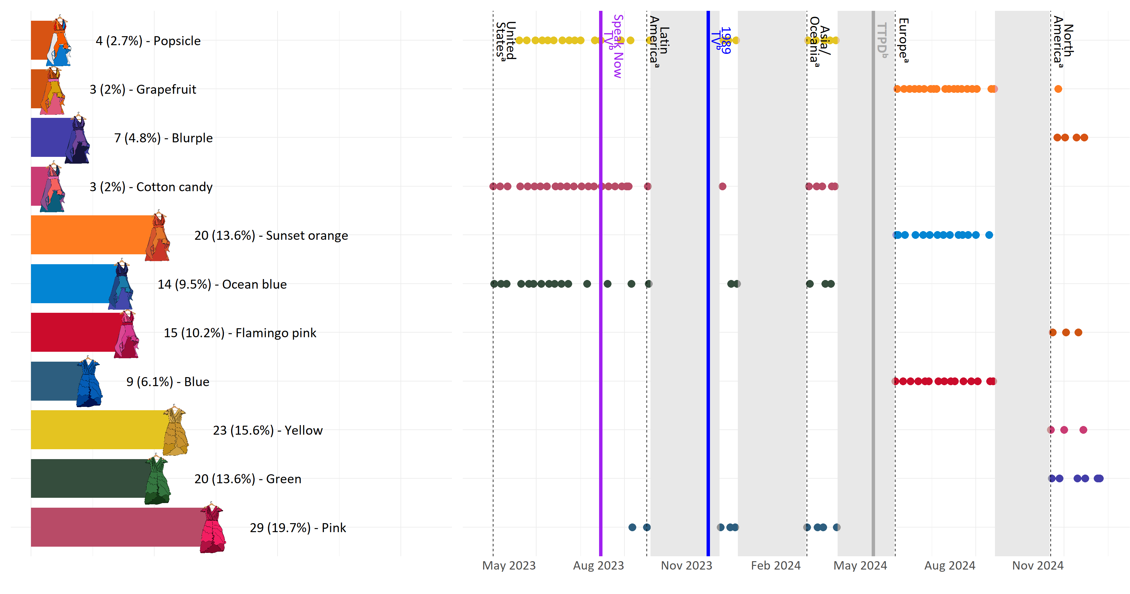

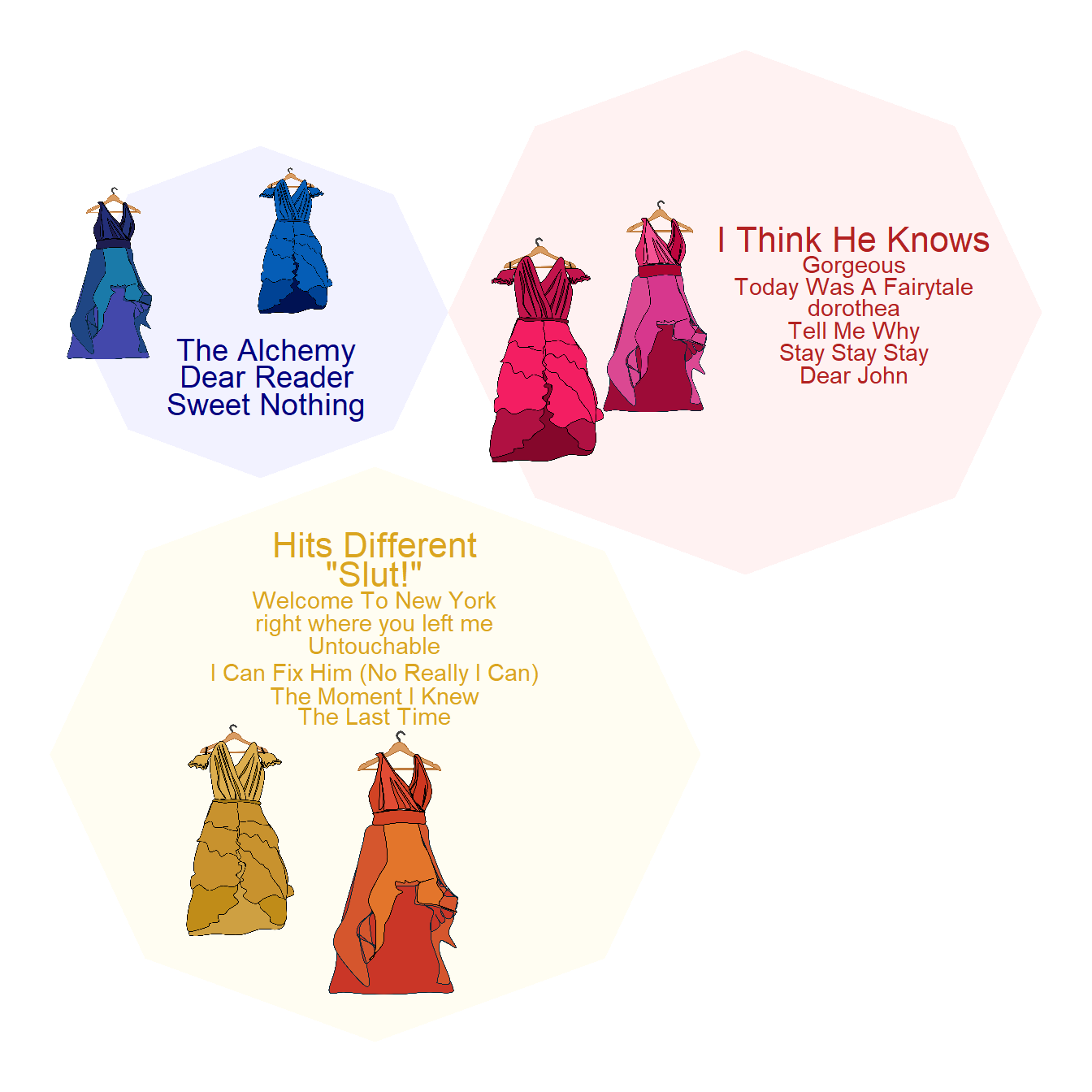
Surprise song color groups

surpriseSongsDressColours$groupName <- sapply(surpriseSongsDressColours$DressName, function(color) {
  if (color %in% c("Pink", "Flamingo pink")) return("reds")
  if (color %in% c("Green")) return("greens")
  if(color %in% c("Yellow", "Sunset orange")) return("yellows")
  if (color %in% c("Ocean blue", "Blue")) return ("blues")
  if (color %in% c("Popsicle", "Cotton candy", "Grapefruit")) return ("colorful")
  if (color %in% c("Blurple")) return("purples")
  return("Neutral")
})

songs_with_single_color_group <- surpriseSongsDressColours %>%
  group_by(`Song title`) %>%
  summarize(
    total_performances = n(),
    unique_color_groups = n_distinct(groupName),
    color_group = first(groupName) 
  ) %>%
  filter(unique_color_groups == 1, total_performances > 1) %>%
  arrange(desc(total_performances))

single_color_performances <- surpriseSongsDressColours %>%
  filter(`Song title` %in% songs_with_single_color_group$`Song title`)

## pics
blues <- paste("dress_drawings/", c("blue", "Ocean blue"), ".png", sep = "")
reds <- paste("dress_drawings/", c("pink", "Flamingo pink"), ".png", sep = "")
yellows <- paste("dress_drawings/", c("yellow", "Sunset orange"), ".png", sep = "")

coords <- circleProgressiveLayout(table(single_color_performances$groupName),
                                  sizetype = 'area')
coords$id <- names(table(single_color_performances$groupName))

df.gg <- circleLayoutVertices(coords, npoints = 8, id = 4)

snames <- single_color_performances %>% select('Song title', groupName) %>%
  group_by(`Song title`) %>% mutate(count = n()) %>% ungroup() |> unique()

set.seed(1989) ## for jitter repel

plot <- ggplot() + theme_void() +
  ## blues
  geom_polygon(data = df.gg[df.gg$id == "blues",], aes(x = x, y = y),
               fill = "#0000FF", alpha = 0.05) +
  geom_text_repel(aes(x = coords$x[coords$id == "blues"], 
                      y = coords$y[coords$id == "blues"], 
                      label = snames$`Song title`[snames$groupName == "blues"]),
                  col = "navy", 
                  nudge_y = -0.5, 
                  nudge_x = 0.05, 
                  segment.color = NA,
                  size = 2.5*snames$count[snames$groupName == "blues"], 
                  box.padding = 0.05,
                  max.overlaps = 30,
                  force = 0.5,
                  direction = "y") +
  ## reds
  geom_polygon(data = df.gg[df.gg$id == "reds",], aes(x = x, y = y),
               fill = "#FF0000", alpha = 0.05)  +
  geom_text_repel(aes(x = coords$x[coords$id == "reds"], 
                      y = coords$y[coords$id == "reds"], 
                      label = snames$`Song title`[snames$groupName == "reds"]),
                  col = "firebrick", 
                  nudge_y = 0, 
                  nudge_x = 0.8, 
                  segment.color = NA,
                  size = 1.9*snames$count[snames$groupName == "reds"], 
                  box.padding = 0.05,
                  max.overlaps = 30,
                  force = 0.5,
                  direction = "y") +
  ## yellows
  geom_polygon(data = df.gg[df.gg$id == "yellows",], aes(x = x, y = y),
               fill = "#FFD700", alpha = 0.05)  +
  geom_text_repel(aes(x = coords$x[coords$id == "yellows"], 
                      y = coords$y[coords$id == "yellows"], 
                      label = snames$`Song title`[snames$groupName == "yellows"]),
                  col = "goldenrod", 
                  nudge_y = 1.2, 
                  nudge_x = 0, 
                  segment.color = NA,
                  size = 1.9*snames$count[snames$groupName == "yellows"], 
                  box.padding = 0.05,
                  max.overlaps = 30,
                  force = 0.5,
                  direction = "y")

# Improved dress scaling - slightly smaller to fit better
get_dress_scale <- function(dress_name) {
  counts <- c("Blue" = 2, "Ocean blue" = 4, "Pink" = 8, 
              "Flamingo pink" = 7, "Yellow" = 7, "Sunset orange" = 11)
  base_scale <- 0.11
  scale_factor <- 0.012
  return(base_scale + (counts[dress_name] * scale_factor))
}

# Final plot with adjusted dress positions
ggdraw() +
  draw_plot(plot) +
  draw_image(blues[1],  -0.23, 0.28, scale = get_dress_scale("Blue")) +
  draw_image(blues[2], -0.4, 0.25, scale = get_dress_scale("Ocean blue")) +
  draw_image(reds[1], 0, 0.18, scale = get_dress_scale("Pink")) +
  draw_image(reds[2], 0.10, 0.22, scale = get_dress_scale("Flamingo pink")) +
  draw_image(yellows[1], -0.28, -0.26, scale = get_dress_scale("Yellow")) +
  draw_image(yellows[2], -0.14, -0.29, scale = get_dress_scale("Sunset orange"))

“Billboard Hot 100™.” n.d. https://www.billboard.com/charts/hot-100/.

Bortoli, Mario De, and Jesús Maroto. 2001. “Colours Across Cultures: Translating Colours in Interactive Marketing Communications.” In European Languages and the Implementation of Communication and Information Technologies (Elicit) Conference.

Kaufman, Gil. 2025. “Orange You Glad Taylor Swift Is Back?” Billboard, August. https://www.billboard.com/music/pop/taylor-orange-life-showgirl-album-memes-elmo-target-brands-1236042681/.

Olson, Samantha. 2022. “All the Easter Eggs in Taylor Swift’s Bejeweled Music Video.” Seventeen, October. https://www.seventeen.com/celebrity/music/a41766334/taylor-swift-bejeweled-music-video-easter-eggs/.

Rinker, Tyler W. 2021. “Sentimentr: Calculate Text Polarity.”

Rowley, Glenn. 2023. “Taylor Swift’s the Eras Tour Easter Eggs: Here’s What Fans Have Spotted.” Billboard, May. https://www.billboard.com/lists/taylor-swift-eras-tour-easter-eggs/the-red-taylors-version-t-shirt/.

Savage, Mark. 2024. “Taylor Swift: As the Eras Tour Bows Out, What Will She Do Next?” BBC, December. https://www.bbc.com/news/articles/ckg1r0v838vo.

Thompson, W Jake. 2025. “Taylor: Lyrics and Song Data for Taylor Swift’s Discography.”